
by Andrew Kliman, author of Reclaiming Marx’s “Capital” and The Failure of Capitalist Production
Around the time of the Occupy movement, and for some time thereafter, discussion of economic inequality in the U.S. tended to focus on inequality of income. More recently, however, attention has increasingly been paid to inequality of wealth.[1] The change in focus is associated with the publication––and the political use––of a shocking paper by Emmanuel Saez and Gabriel Zucman (2016), which diverged sharply from the consensus view among other researchers. According to the consensus view, wealth inequality had increased only modestly in recent decades. In marked contrast, Saez and Zucman reported that the share of wealth held by the top 1% of the population rose by more than 80% between 1978 and 2012, and that the share held by the top 0.1%––the wealthiest tenth of “the 1%”––more than tripled.[2]
Even though their study is extremely controversial, Saez and Zucman’s conclusions have been endorsed and widely publicized by politicians such as Senators Bernie Sanders and Elizabeth Warren, as well as by some journalists and political commentators. In June 2015, when announcing his proposed legislation to increase estate-tax rates and eliminate loopholes in the current law, Sanders (2015) justified the bill by appealing to “the most recent statistics”––that is, to the Saez-Zucman study. More recently, both Sanders and Warren have called for a wealth tax to be levied on the super-rich; and both Saez and Zucman have been serving as advisors to Warren.
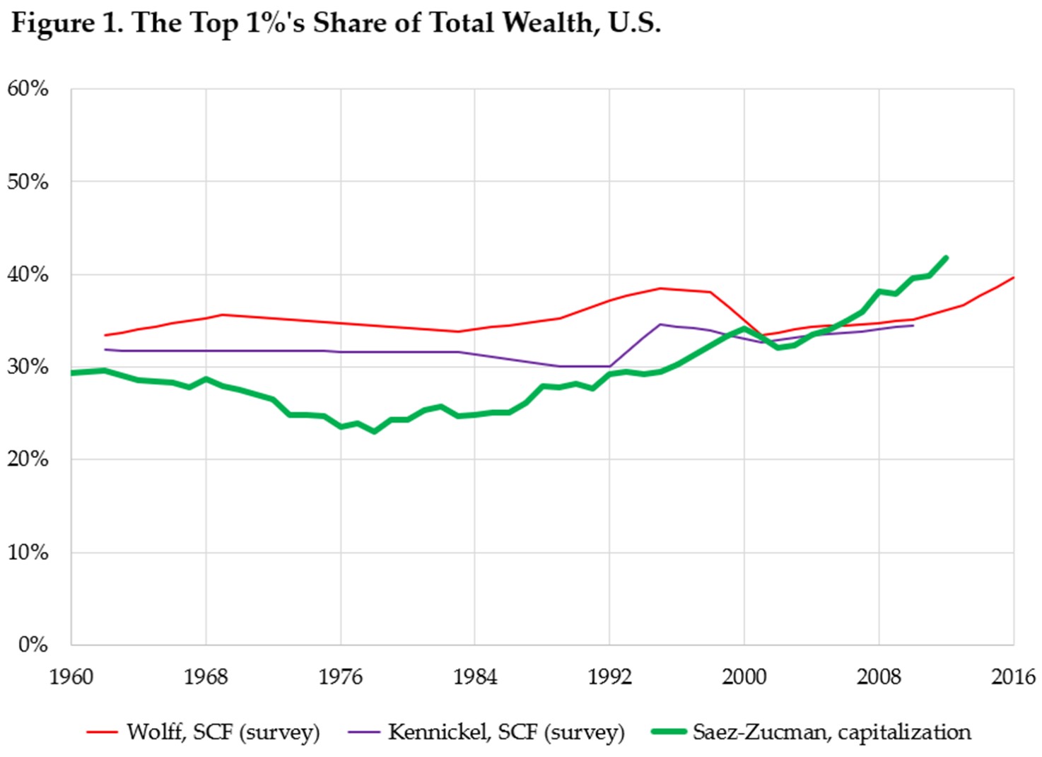
The consensus view of wealth inequality in the U.S. is based mostly on studies that use data reported in the Federal Reserve Board’s Survey of Consumer Finances (SCF). The SCF data are obtained from in-person and telephone interviews in which respondents detail their various assets and liabilities. This approach leads to the conclusion that between 1983 and 2007––which is roughly the period of pre-Great Recession “neoliberalism”––wealth inequality increased only modestly. For example, Arthur Kennickel (2012), who used data from the SCF data and similar precursor surveys, estimated that the share of total wealth held by the top 1% of the population rose by just 2.2 percentage points during this period (see Figure 1.)[3] Edward N. Wolff (2017), who used the same data but excluded ownership of vehicles from his definition of wealth, estimated that the rise was even smaller, 0.8 percentage points.
Saez and Zucman took a different approach. Instead of using actual wealth data provided by survey respondents, they principally used income data reported on tax returns to estimate holdings of wealth. Specifically, they took data on capital income and “capitalized” it.[4] In marked contrast to the studies based on survey data, this variant approach leads to the conclusion that wealth inequality increased throughout the entire period of pre-Great Recession “neoliberalism,” 1983–2007. It also leads to the conclusion that the increase in wealth inequality was much greater than survey-based studies suggest. Saez and Zucman’s figures imply that the top 1%’s share of wealth skyrocketed by 11.2 percentage points over this period, which is more than 5 times as big as the rise reported by Kennickel, and more than 14 times as big as the rise reported by Wolff.
Wealth Inequality: Level and Kind versus Trend
All of these studies found the distribution of wealth in the U.S. to be enormously unequal. And this is nothing new. We now have two different studies that extend back more than a century, both of which conclude that wealth has been distributed exceedingly unequally the whole time. Using estate-tax data to estimate wealth, Kopczuk and Saez (2004) found that the share of total wealth held by the top 1% of the population was, on average, 37.0% from 1916 to 1930, 27.2% from 1931 to 1945, and 22.3% from 1946 to 2000. For the same subperiods, Saez and Zucman’s estimates of the top 1%’s share of wealth were 42.1%, 41.3%, and 28.1%.
Another way of thinking about these numbers is to compare the wealth of an average household in the top 1% to the wealth of an average household in the rest of the population. Kopczuk and Saez’s figures imply that top 1% households were, on average, 58 times as wealthy as other households from 1916 to 1930, 37 times as wealthy from 1931 to 1945, and 28 times as wealthy from 1946 to 2000. Saez and Zucman’s figures imply that they were 72, 70, and 39 times as wealthy, during the same subperiods.
The Kopczuk-Saez (2004) study found the distribution of wealth to be somewhat more equal than did the Saez-Zucman study. In this respect, it is the Kopczuk-Saez paper that is the exception. As Figure 1 showed, studies based on the SCF and precursor surveys conclude that the degree of wealth inequality during the last four decades of the 20th century was greater than the degree that Saez and Zucman’s figures suggest.
Thus, the key difference between the Saez-Zucman study and the consensus view of other researchers does not pertain to the level of wealth inequality. It instead pertains only to its trend––the amount by which wealth inequality has risen and when the rise began.
When advocating policies that are intended to reduce the inequality of wealth, it would be perfectly reasonable to point to the level of inequality rather than its trend. In other words, one could reasonably justify such policies on the grounds that the current distribution of wealth is so enormously unequal, rather than on the grounds that inequality of wealth has been rising sharply. For one thing, the former justification is based on an uncontested fact, while the latter one is not.
It is noteworthy, then, that Sanders and Warren have chosen to lean so heavily on the controversial claim that inequality of wealth has skyrocketed. When introducing his 2015 estate-tax bill, Sanders (2015) said that
… if we do not make the necessary changes to reduce skyrocketing wealth and income inequality, this country, in my view, is well on its way to becoming an oligarchic form of society …. [Wealth and income] inequality is worse today than at any time since 1928. We are moving in exactly the wrong direction. The fact of the matter is, that over the past 40 years, we have witnessed an enormous transfer of wealth from the middle class and working families of our country to multi-millionaires and billionaires.
And when she announced her proposed wealth tax, Warren (2019) justified it in the following manner:
For decades, a small group of families has raked in a massive amount of the wealth American workers have produced, while America’s middle class has been hollowed out. The result is an extreme concentration of wealth not seen in any other leading economy. According to an analysis from economists Emmanuel Saez and Gabriel Zucman from the University of California-Berkeley, the richest top 0.1% has seen its share of American wealth nearly triple from 7% to 20% between the late 1970s and 2016, while the bottom 90% has seen its share of wealth decline from 35% to 25% in that same period.
Even if we were to assume, for the sake of argument, that there is adequate evidence that wealth inequality has skyrocketed, it is hard to see that one provides better justification for a proposal to redistribute wealth by pointing to this trend instead of by pointing to the simple fact that the level of wealth inequality is so enormous. Nonetheless, focus on the trend instead of the level has some political advantages for those who practice a certain kind of politics, namely left economic populism. (To others of us, these political advantages are disadvantages).
By pointing to a sharply rising trend in wealth inequality since the late 1970s, one places the blame on one’s political opponents––neoliberals, centrists, pro-establishment types. One certainly does not blame the Keynesians, supporters of the New Deal, or the rest of the pre-neoliberal consensus that countenanced a distribution of wealth that was massively lopsided even before it trended upward. And by concentrating on the (purported) trend, one focuses on a secondary aspect of wealth inequality that tax manipulation and other redistributive measures may be able to ameliorate, instead of the primary problem––the massive level of wealth inequality––that will persist even after redistributive measures have done what they can do.
Above all, one does not implicate the capitalist system itself, even though the system itself is directly responsible for the lion’s share of wealth inequality. Capitalist relations of production––the split between owners of productive wealth (capital) and proletarians who have little if any productive wealth of their own––began when the English peasants were driven off of their land about 400-500 years ago (Marx 1990, chap. 27). And this separation of the great majority of working people from productive wealth is continually renewed. By scrimping and saving, they may be able to own houses and cars, to put aside money for their retirement years, and, in some cases, to have a little extra that they can leave to their children. But only in the most exceptional cases can they save or borrow enough to escape the choice of either starving or being compelled to work for others and under the direction of others. Thus, a proletariat separated from productive wealth persists year after year, generation after generation. It is this dynamic, precisely this, that is responsible for both the lion’s share of wealth inequality and the continuing existence of capitalist relations of production.
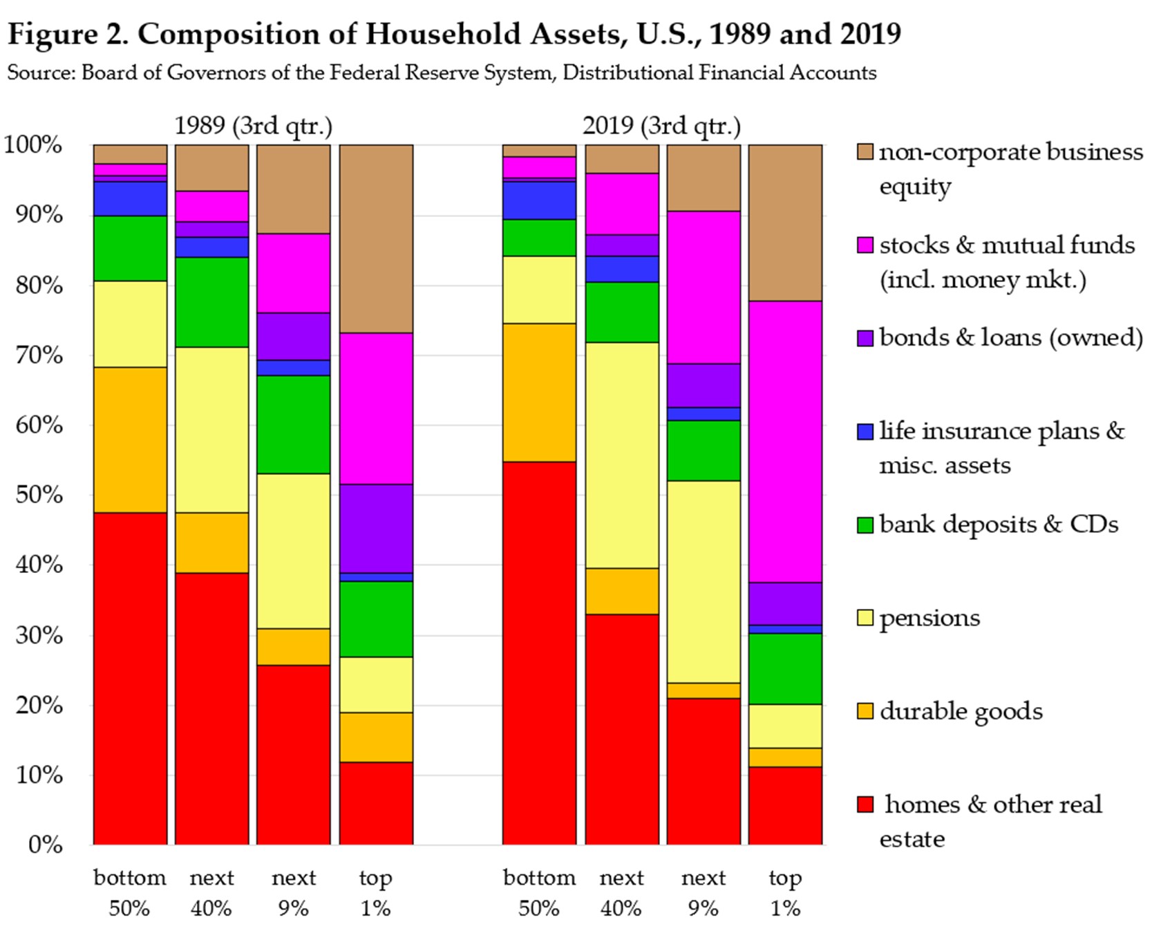
Indeed, as Figure 2 shows, the kinds of “wealth” held by working people in the U.S.––especially those in the least-wealthy half of the population, but also the 40% of the population above that––are extremely different from the kinds of wealth held by those at the top. The overwhelming majority of the “wealth” of the bottom 90% of households consists of the homes they live in, the cars and other durable goods they use, their pensions for their retirement years, and relatively small amounts of funds in banks and life-insurance policies.[5]
The figures are for the past three decades. The available statistics do not go back further, but it is quite hard to imagine that the bottom 90% held substantial amounts of productive wealth before then.
Only about 5% of the “wealth” of those in the bottom half, and about 15% of the “wealth” of the next 40%, has consisted of ownership of businesses—either directly or through ownership of corporate stock—and bonds. In contrast, between 60% and 70% of the wealth of the top 1% of households, and about one-third of the wealth of the next-wealthiest 9%, has consisted of ownership of businesses and bonds.
Figure 3 shows the dollar amounts of the bottom 90%’s business, stock, and bond assets. Their average holdings of these forms of wealth almost doubled between 1989 and 2019, but the increase since 2010 has been driven almost entirely by rising stock prices. The bottom 90%’s holdings of non-corporate businesses and bonds have basically been constant, in real terms, since 2010.[6]
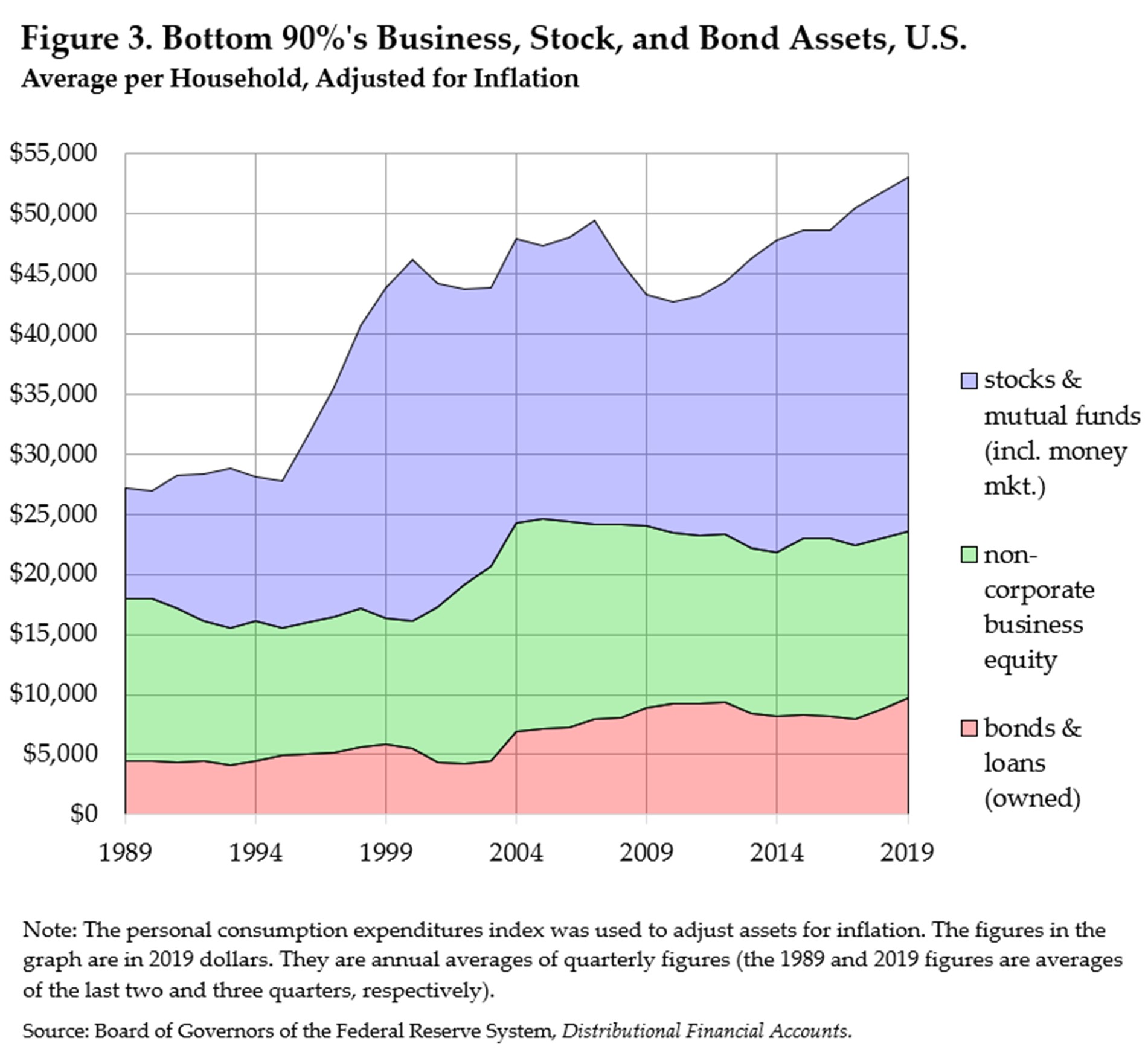
Even though their business, stock, and bond assets have almost doubled, the total amount of these assets owned by the bottom 90% of the population was still only $53,000 per household as of last year. This is far less than one year of income for a household at the median. It certainly is nowhere near the amount of wealth that the people in that household would need to extricate themselves from the continual compulsion to work for, and under the direction of, others. And among the bottom half of the population, last year’s per-household business, stock, and bond assets totaled less than $6000!
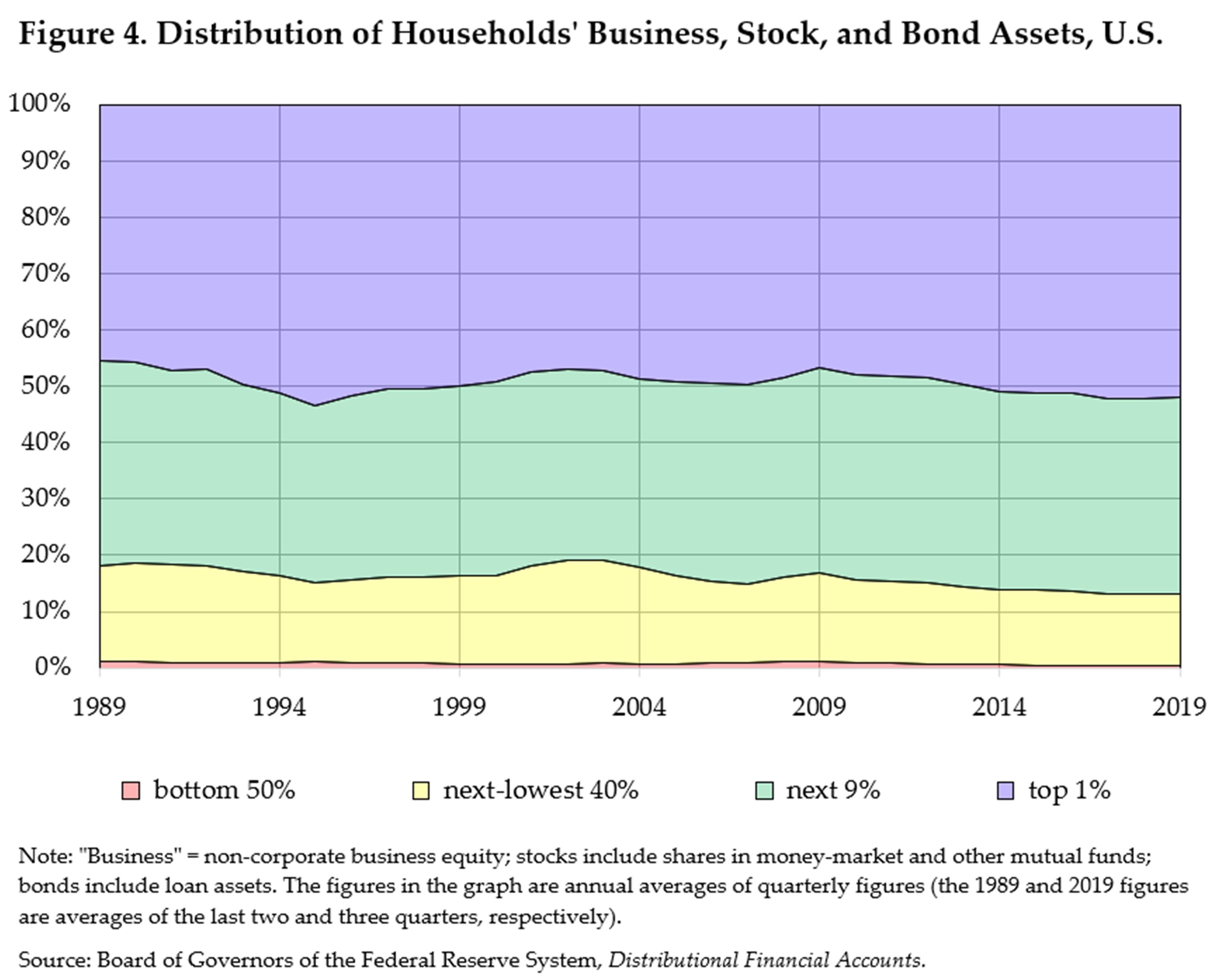
Figure 4 shows how non-corporate business, stock, and bond assets are distributed among households. Over the last 30 years, almost half (49% on average) of this wealth has been in the hands of the top 1%, and a little more than one-third (35%) has been owned by the next-wealthiest 9% of households. The bottom half of the population has owned almost none of it (1%), and the next-lowest 40% of households have owned only about 15%. Prior to the Great Recession, these shares were remarkably stable; none of them trended upward or downward to a substantial degree. Since 2009, however, the top 1%’s share has risen by about 5 1/2 percentage points, while the shares of these forms of wealth owned by all of the other groups have declined, especially the share owned by the 40% of the population immediately above the bottom half.
Wealth of the Median Household
There is an additional reason that it is inappropriate to put too much emphasis on the trend (if any) in the inequality of wealth: a rise in wealth inequality does not imply that the poor are becoming poorer. Unfortunately, political rhetoric often seems to be based on the idea that this is precisely what it does imply. Recall, for instance, that when he announced his estate-tax bill, Bernie Sanders said that “over the past 40 years, we have witnessed an enormous transfer of wealth from the middle class and working families of our country to multi-millionaires and billionaires” (emphasis added). The claim that wealth has been transferred upward is, at best, quite misleading.
Of course, if the total stock of wealth had remained constant, then the very rich could capture a bigger share of the total only if a portion of the wealth held by the rest of the population were transferred to them––in other words, they could become wealthier only if the rest of the population became poorer. But the total stock of wealth has not remained constant. It has increased rather rapidly, and non-wealthy households have captured a portion of the extra wealth. They have thus become wealthier, not poorer. (It bears re-emphasizing, however, that most of the “wealth” of the working class consists of the homes they live in, the cars they drive, and the money they save up for their retirement years.) The share of wealth held by the very rich has increased, not because they have wrested away some of the wealth that formerly belonged to the rest of the population, but because their share of the extra wealth has been especially large.
Figure 5 shows how the wealth of the median (middle) household has changed since 1962. It is based on data reported in the SCF for the 1989-2016 period, and on estimates of mine for 1962, 1969, and 1983 that employ median-wealth figures reported in Wolff (2017), which are based on the SCF and on similar precursor surveys.[7] The median wealth figures are in “real” terms, adjusted for inflation by means of the Consumer Price Index research series using current methods (CPI-U-RS). Thus, when median wealth doubles, this means that the median household’s wealth can purchase twice as much “real stuff” (rather than, say, the same amount of stuff at prices that have doubled).
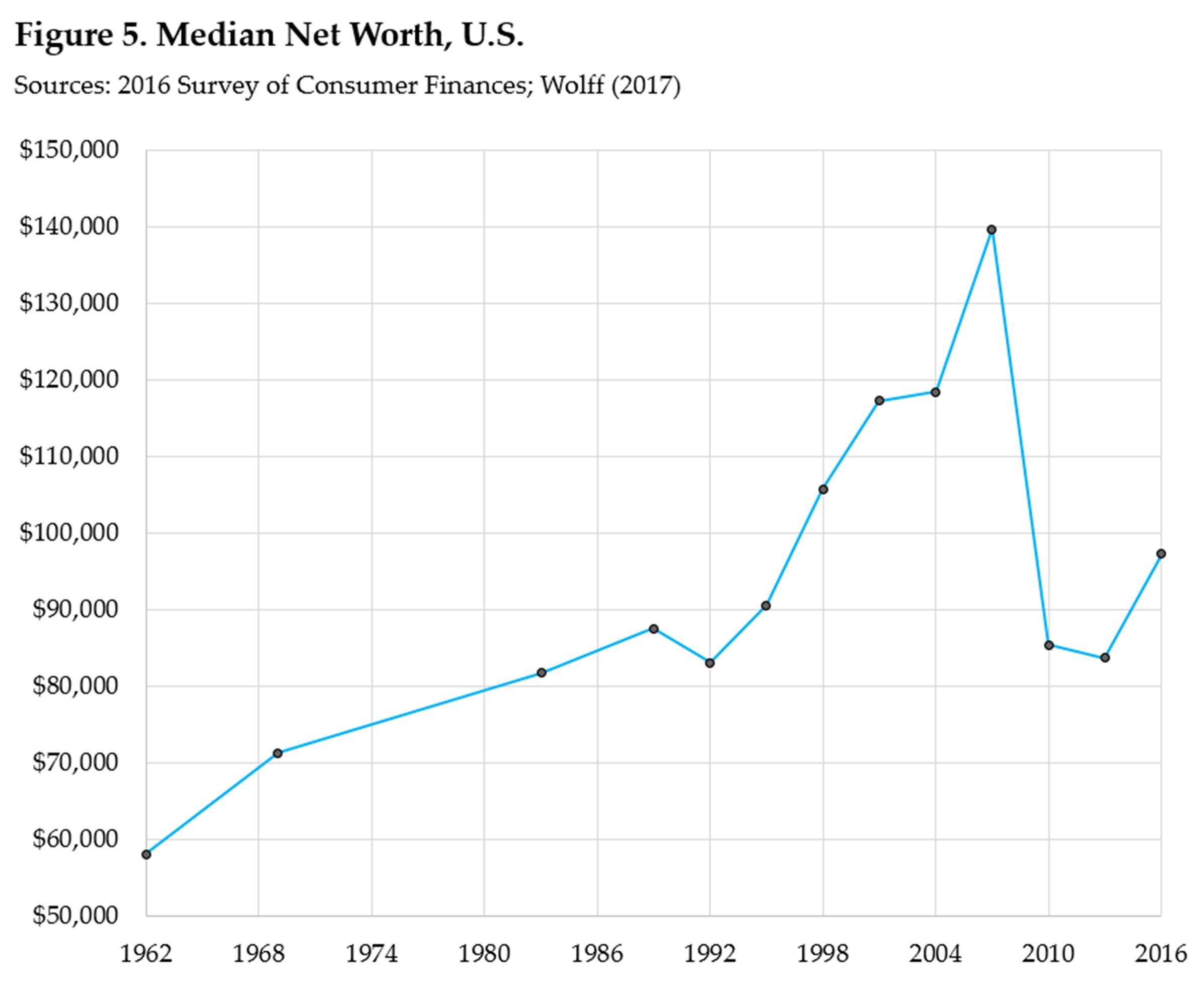
Between 1962 and 1983, the median household’s wealth increased, on average, by 1.9% per year. Between 1983 and 2007, the period of pre-Great Recession “neoliberalism,” its wealth increased even more rapidly, by 3.0% per year. It then lost two-fifths of its wealth during the Great Recession and its aftermath. As of 2016, it had recovered less than one-fourth of that lost wealth.
One of the main reasons median wealth plummeted so sharply during the recession was that home prices collapsed. The collapse had a particularly large impact on the wealth of the middle class because homes are its largest asset, by far. The other main reason is that, at the onset of the recession, the debt of the middle class was very large in relation to its assets, so that the fall in its assets caused its net worth to decline by a much larger percentage than it would have declined if its debt had initially been small in relation to its assets.[8]
It seems very unlikely that the rise in median wealth prior to the Great Recession can be attributed to the fact that the data come from the SCF rather than from the Saez-Zucman study. Saez and Zucman did not provide median wealth data, nor can median wealth be computed from the numbers in their data set, but they did report a somewhat similar statistic: the real average wealth of the bottom 90% of the population. It increased by 3.2% per year, on average, between 1962 and 1983, and by 3.6% per year between 1983 and 2007.[9] It thus appears that there was sizable growth in the real wealth of households that were roughly in the middle of the distribution––irrespective of whether wealth inequality is said to have increased rapidly or to have increased only slowly.
But Who is Right about the Trend?
Saez and Zucman justify their effort to estimate wealth by means of tax-return income data, instead of using actual wealth data, by arguing that the SCF fails to adequately measure the wealth of the super-rich: the percentage of the super-rich who respond to the survey is exceptionally small, and the survey also excludes almost all of the very wealthiest people (the Forbes 400) from its sample. Yet the SCF deals with the under-response problem by including a disproportionate share of super-rich households in its sample, and papers written by Federal Reserve economists (Kennickel 2009, p. 19; Bricker, et al. 2015, pp. 6–7) find very little evidence to suggest that the super-rich people who do respond to the survey are unrepresentative of the group in general. Bricker, et al. (2015) also adjust the FCP data so as to include Forbes 400 households, and they find that the adjustment has very little effect on the trend in wealth inequality.
There are many reasons to be skeptical of Saez and Zucman’s estimates. Some of the problems are also present in the famous and much-celebrated work on income inequality that Saez and Zucman have done with Thomas Piketty, since they are problems inherent in the use of tax-return data to assess inequality.
“Tax Units”
One such problem is that the Saez-Zucman figures do not actually refer to individuals (or households or families). They refer to “tax units” (see Kliman 2013). Owing to a long-term decline in the marriage rate, the number of tax units has grown more rapidly than the number of individuals (since a married couple is one tax unit while an unmarried couple is two). But there has been little decline in the marriage rate of the super-rich, so the excess growth of tax units relative to individuals is concentrated in the rest of the population––“the 99%.” Thus, among “the 99%,” growth of wealth (and income) per tax unit has increasingly fallen in relation to growth per individual. In this way, figures based on tax units artificially reduce the shares of wealth and income that “the 99%” receive, thereby artificially boosting the shares of “the 1%,” and the artificial rise in inequality gets larger with each decline in the marriage rate.
Inconsistencies Due to Changes in Tax Law
Another problem inherent in the use of information reported on income-tax returns is the fact that it results in inconsistent data sets, because “taxable income” does not have the same meaning over time. It changes as tax laws change and as people and companies respond to changes in the laws. Consequently, a rise in the “income” of the super-rich may signify that they are reporting more of their income on tax returns, not that their income has actually risen.
Consider, for example, the sharp rise, between 1986 and 1988, in the Saez-Zucman data series shown in Figure 1. The share of wealth held by the top 1% supposedly rose by 2.8 percentage points, which is more than a fifth of the total rise in this data series between 1978 and 2007. This increase in wealth reflects an increase in income––owing to Saez and Zucman’s use of the latter to estimate the former––and this sharp rise in the “income” of the top 1% coincided with the Tax Reform Act of 1986 (TRA86). Little of that rise reflects a genuine increase in the income of the super-rich; most of it stems from super-rich business owners merely shifting their existing income in response to TRA86.
Reversing the pre-existing situation, TRA86 set the tax rate on individual income at a level lower than the tax rate on corporate income, thereby creating an incentive for super-rich business owners to report more of their income as individual income instead of corporate income––by turning C-corporations into S-corporations and by other means.[10] As a result, the number of businesses that elected to become S-corporations during the last three weeks of 1986 was triple the number that elected to do so during the whole of 1985 (Feenberg and Poterba 1992, p. 156). Since Saez and Zucman ignore corporate income but count individual income, they treat this shift in income as if it were a genuine increase.
TRA86 may also have led to greater reporting of income because it limited deductions for losses on rental income and passive investments. And there are reasons to suspect that the effect of TRA86, and other changes in tax laws, on reported income was not merely temporary. One reason is that Piketty and Saez’s top 1% income share has continued to rise more sharply than income shares that are not derived primarily from tax records.
Gerald Auten and David Splinter (2019) address the shift away from the C-corporation form of ownership by assuming, in effect, that it did not exist in the first place. They do so by counting corporations’ retained profit as if it were individual income that passes through to the corporations’ owners. And for the same reason, they count income taxes paid by corporations as part of the owners’ pre-tax individual income. These two adjustments substantially reduce the growth of income of the top 1%. Between 1978 and 2012, for instance, Saez and Zucman’s figures indicate that the top 1%’s income rose, on average, by 12.7% per year (after correcting for inflation). After the two adjustments made by Auten and Splinter, the rise is reduced by one-fourth, to 9.6% per year.[11]
Capitalization as Guesstimation
Use of the capital-income figures that appear in tax returns––which Saez and Zucman rely on to estimate wealth––is problematic for other reasons as well. One problem is that about two-thirds of capital income does not appear on tax returns; it must be estimated (Kopczuk 2015, pp. 54–55). Another problem is that, because capital gains are taxed at a lower rate than other income, wealthy individuals have a strong incentive to file tax returns that report some of their labor income as capital income (ibid., pp. 55–56).
Furthermore, the estimation of wealth from capital income is fraught with problems. In principle, it is straightforward––one “capitalizes” a flow of capital income by dividing the income by the associated rate of return. The quotient is the value of the asset that generated the income.[12] In other words, given the rate of return, the quotient is the amount of wealth that was needed in order to generate the flow of capital income. The problem, however, is that rates of return are frequently unknown. They must be estimated. In some cases, the estimated rates of return are essentially just guesstimates, or even numbers that, although obviously wrong, suffice to dispose of an intractable estimation problem.
Fixed-Income Assets: Checking Deposits = High-Yield Bonds?
For example, Saez and Zucman assume that all fixed-income assets yield the same rate of return, even though the fixed-income category includes everything from checking and savings deposits to the myriad of bonds, each of which has its own interest rate. Similarly, they assume in effect that all owners of the same kind of asset receive the same rate of return on that asset, even though people frequently become super-rich precisely because they obtain extraordinarily high rates of return on their investment. “Obvious examples include [investors in] successful technology companies––say Microsoft, Apple, or Google––that made their owners into billionaires” (Kopczuk 2015, p. 56).
These rate-of-return estimation problems can greatly affect the measured degree of wealth inequality. Wealthy people obtain higher rates of return than the rest of the population––because they struck it rich, because their fixed-income assets are disproportionately bonds rather than bank accounts (Smith, Zidar, and Zwick 2019, p. 14),[13] and so on. When one assigns a too-low rate of return––for example, some average rate––to their assets, the capitalization formula overestimates the value of the assets, making the wealthy seem even wealthier than they are. Conversely, use of an average rate will assign a too-high rate of return to the assets of the rest of the population, and thereby make it seem less wealthy than it is. And if rates of return fall, but the rates that the wealthy actually receive fall less sharply than the average rate of return, then the capitalization formula will produce a spurious increase in the inequality of wealth.
The majestic equality of Saez and Zucman’s procedure for estimating fixed-income assets, which prohibits the rich and the poor alike from obtaining high rates of return on them, has come under considerable, and sustained, scrutiny. This is because they report a much larger rise in wealth inequality in recent years than other studies do, and the valuation of fixed-income assets turns out to be a large source of the difference, since “nearly all of the growth in recent years in the capitalized top 0.1 share arises from the growth in fixed-income assets” (Bricker, et al. 2015, p. 19).
Critics of Saez and Zucman’s work have explored the implications of discarding their assumption that rates of return on fixed-income assets are equal. They have assumed, instead, that the rate of return received by wealthy households has been greater––to a degree that they, although not Saez and Zucman (2016, pp. 550–51; 2020), deem to be reasonable.[14] It turns out that this adjustment to the Saez-Zucman data eliminates a good deal of the difference between their estimate and other studies’ estimates of the rise in wealth inequality in recent years (Bricker et al. 2015; Bricker, Henriques, and Hansen 2018; Smith, Zidar, and Zwick 2019).
Owner-occupied Housing
Saez and Zucman’s valuation of owner-occupied housing is also a source of controversy. In the SCF, the value of owner-occupied housing is based on the information that survey respondents provide. But in the Financial Accounts of the United States that Saez and Zucman use, its value is estimated by means of a “perpetual inventory” formula rather than direct evidence. Bricker, et al. (2015, Figure 10) show that, in 1995, the aggregate SCF value was about 5% larger than the aggregate Financial Accounts value, but by 2010, it had become more than 40% larger. The difference has a big effect on the wealth-distribution numbers, since owner-occupied housing wealth is a large component of total assets that is also much more equally distributed than wealth in general. Thus, if the survey information is correct, use of the Financial Accounts figures has led to a substantial undervaluation of owner-occupied homes; this error has depressed the estimated wealth of the population in general to a much larger degree than it has depressed the estimated wealth of those at the top, thereby producing a spurious increase in wealth inequality; and the effect of this error has increased over time (Bricker, et al. 2015, p. 17).
In Lieu of a Conclusion
Although there are several good reasons to take the findings of Saez and Zucman with a grain––or even a pillar––of salt, I cannot draw a definitive conclusion regarding who is right about the trend in U.S. wealth inequality. The debate is still taking place; Saez and Zucman’s (2020) response to Smith, Zidar, and Zwick (2019) came out just two weeks ago. And to adequately come to grips with some of the issues now under contention, one needs more than a solid understanding of income and wealth distribution. One needs very specialized expertise regarding details of tax records and official financial accounts, and considerable time to devote to fine points of extremely detailed statistical studies, neither of which I have.
Yet there is one thing that is indeed clear, precisely because the debate is still ongoing and unresolved: it is intellectually irresponsible for researchers to treat their studies on the trend in wealth inequality as having established uncontested facts (Saez and Zucman 2019a, p. 4). And it is intellectually irresponsible for politicians, journalists, and commentators to follow them down that road. It may serve well as post-truthy populism, but, in this era of Trumpism, one of the main threats to us is post-truthy populism itself.
I concur with the comment recently made by Wojciech Kopczuk (who co-authored Kopczuk and Saez (2004) with Saez). The Saez-Zucman wealth estimates, Kopczuk (2019, p. 8) writes, “are highly uncertain numbers that should be presented together with some explicit notion of the magnitude of the measurement error. … All sources of information point to an increase in wealth inequality. Exactly how much is very much uncertain and should not be presented as certain.”
Whether wealth inequality has risen sharply, modestly, or not at all, several facts about the level of wealth inequality are also clear. It is massive. Its main source is capitalism itself––the separation of working people from productive resources of their own. And the perpetuation of the capitalist system requires that the inequality of wealth remain massive.
But the perpetuation of capitalism is not a given. Another world is possible. The struggle continues.
References
Auten, Gerald and David Splinter. 2019. Income Inequality in the United States: Using Tax Data to Measure Long-term Trends. Working Paper, Dec. 20.
Bricker, Jesse, Alice M. Henriques, Jake A. Krimmel, and John E. Sabelhaus. 2015. Measuring Income and Wealth at the Top Using Administrative and Survey Data. Finance and Economics Discussion Series 2015-030, April. Washington: Board of Governors of the Federal Reserve System.
Bricker, Jesse, Alice Henriques, and Peter Hansen. 2018. How much has wealth concentration grown in the United States? A re-examination of data from 2001-2013. Finance and Economics Discussion Series 2018-024, March 30. Washington: Board of Governors of the Federal Reserve System.
Feenberg, Daniel R. and James M. Poterba. 1993. Income Inequality and the Incomes of Very High-Income Taxpayers: Evidence from Tax Returns. In James M. Poterba (ed.), Tax Policy and the Economy, Volume 7, pp. 145–177. Cambridge: The MIT Press.
Kennickell, Arthur B. 2009. Getting to the Top: Reaching Wealthy Respondents in the SCF, August 18. Paper prepared for the 2009 Joint Statistical Meetings, Washington.
_______. 2012. Tossed and Turned: Wealth Dynamics of U.S. Households 2007–2009. Finance and Economics Discussion Series 2015-11, May 29. Washington: Board of Governors of the Federal Reserve System.
Kliman, Andrew. 2013. “The 99%” and “the 1%” … of What?, With Sober Senses, Feb. 19.
Kopczuk, Wojciech. 2015. What Do We Know about the Evolution of Top Wealth Shares in the United States?, Journal of Economic Perspectives 29:1, pp. 47–66.
_______. 2019. Comment on “Progressive Wealth Taxation” by Saez and Zucman, November.
Kopczuk, Wojciech and Emmanuel Saez. 2004. Top Wealth Shares in the United States, 1916–2000: Evidence from Estate Tax Returns, National Tax Journal 57:2, Part 2, June, pp. 445–487.
Marx, Karl. 1990. Capital: A Critique of Political Economy, vol. 1. London: Penguin Books.
Saez, Emmanuel and Gabriel Zucman, 2016. Wealth Inequality in the United States since 1913: Evidence from Capitalized Income Tax Data, Quarterly Journal of Economics 2016, 131:2, pp. 519–578.
_______. 2019a. [Letter to Senator Elizabeth Warren], Jan. 18.
_______. 2019b. Progressive Wealth Taxation. Draft conference paper, Brookings Papers on Economic Activity, Sept. 4.
_______. 2020. Comments on Smith, Zidar and Zwick (2019), Jan. 24.
Sanders, Bernie. 2015. Sanders Proposes Bill to Reduce Wealth Inequality. YouTube video, June 25.
Smith, Matthew, Owen Zidar, and Eric Zwick. 2019. Top Wealth in the United States: New Estimates and Implications for Taxing the Rich, July 19. This paper is “preliminary and in progress.”
Warren, Elizabeth. 2019. Senator Warren Unveils Proposal to Tax Wealth of Ultra-Rich Americans, Jan. 24.
Wolff, Edward N. 2014. Household Wealth Trends in the United States, 1962-2013: What Happened over the Great Recession? NBER Working Paper No. 20733, Dec. Cambridge: National Bureau of Economic Research.
_______. 2017. Household Wealth Trends in the United States, 1962 to 2016: Has Middle Class Wealth Recovered? NBER Working Paper No. 24085, Nov. Cambridge: National Bureau of Economic Research.
Notes
[1] A household’s wealth, also known as its net worth, is a “stock,” the sum total of the assets it has accumulated over time, minus its outstanding liabilities (loans, etc.). Generally, wealth is defined so as to include not only stocks, bonds, and other financial assets, but also homes and major durable goods. In contrast, income is a “flow.” The portion of current income that a household does not consume (use to purchase consumption goods and services)––but instead saves, or uses to purchase assets or pay down debt––“flows” into its stock of wealth, augmenting it.
[2] These figures come from the “DataFig1-6-7b” sheet of the “Main data” Excel file accompanying their paper.
[3] The data in Figure 1 come from Table 5 on p. 15 of Kennickel (2012); Table 2, Panel A on p. 44 of Wolff (2017); and the “DataFig1-6-7b” sheet of the “Main data” Excel file accompanying Saez and Zucman (2016). The survey-based studies (Kennickel and Wolff) report data only for 1962, 1969, 1983, and for every third year from 1989 onward; I used linear interpolation to estimate the top 1%’s shares in intervening years.
[4] Capitalization is explained below, in the “Capitalization as Guesstimation” subsection of the “But Who is Right about the Trend?” section.
[5] Figures 2 through 4 use data reported in the Federal Reserve’s new Distributional Financial Accounts.
[6] To adjust for inflation, I used the price index for personal consumption expenditures reported on line 2 of Table 1.1.4 of the National Income and Product Accounts, published by the Department of Commerce’s Bureau of Economic Analysis. The estimated numbers of households in the bottom 90% are 0.9 times the figures reported in Table HH-1 of the Current Population Survey. Where two population estimates are reported for a single year, the revised estimate was used.
[7] The figures for the 1989-2016 period come from the “Median value of net worth for families with holdings: For all Families” page, in the “Net Worth” section of the SCF Chartbook that accompanies the 2016 SCF (page numbers are not given). To estimate median wealth in earlier years, I used the SCF figure for 1989 and percentage growth rates of median wealth (between 1962 and 1969, 1969 and 1983, and 1983 and 1989) that I computed using the median-wealth figures reported in Table 1 of Wolff (2017). Wolff’s definition of wealth is similar to, but slightly different from, the definition employed in the SCF, so I concluded that it was safe to use his growth rates to backcast the SCF data series, but not safe to use his median-wealth figures directly alongside SCF figures for later years.
[8] See Wolff (2014, pp. 28-29) for simple numerical examples that clarify how the relation between debt and assets affects the percentage decline in net worth when assets fall.
[9] These figures come from Table B3 of the “Appendix Tables (Distributions)” Excel file accompanying their paper, which is contained in the “Complete data” zip file.
[10] Only C-corporation income is reported on corporate tax returns. Other businesses, including S-corporations and LLCs, are “pass-through entities” that pay no income tax. Their income “passes through” to their owners, who report it on their individual tax returns.
[11] Actually, Auten and Splinter make a great many adjustments to the income figures that Saez and Zucman used, but only these two pertain to the effects of the shift away from the C-corporation form of business organization. The computations are mine, based on data contained in the “C1-Income” sheet and––to adjust for inflation––the personal consumption expenditures (PCE) series provided in the “C0-Ref Stats” sheet of the Excel file accompanying the Auten-Splinter paper. Before eliminating the effect of inflation, the unadjusted income of the top 1% is reported in the leftmost panel of the “C1-Income” sheet; the effect of the two adjustments discussed here is the difference between the Ei2 and Ei0 figures for the top 1%; and their post-adjustment income is the sum of this difference and the top 1%’s unadjusted income.
[12] For example, if interest income is $1000 and the interest rate (the rate of return on the interest-bearing asset) is 4%, then the value of the asset is $1000/0.04 = $25,000. To verify this, note that $25,000 invested at 4% interest generates interest income of $1000.
[13] Summarizing data for 2013, Smith, Zidar, and Zwick (ibid.) write, “The top 0.1% hold just 20% of their fixed income portfolio in liquid assets and bank deposits. Bonds and fixed income mutual funds account for nearly 60%. In contrast, the bottom 99% hold nearly 70% of their fixed income assets in the form of bank deposits.”
[14] However, Saez and Zucman (2019b) have recently conceded that capitalization of fixed-income assets should reflect the fact that the wealthy obtain above-average interest rates, and they have corrected their previous estimates accordingly. They report (ibid., p. 10) that, for recent years, the correction cuts the fixed-income assets of the top 0.1% in half, and that, for 2016, it lowers the fixed-income share of the top 0.1%’s total assets by more than one-third (from 42% to 26%).

Be the first to comment